Model tuning via grid search

tune_grid() computes a set of performance metrics (e.g. accuracy or RMSE) for a pre-defined set of tuning parameters that correspond to a model or recipe across one or more resamples of the data.

Usage

tune_grid(object, ...)

# S3 method for model_spec
tune_grid(
  object,
  preprocessor,
  resamples,
  ...,
  param_info = NULL,
  grid = 10,
  metrics = NULL,
  eval_time = NULL,
  control = control_grid()
)

# S3 method for workflow
tune_grid(
  object,
  resamples,
  ...,
  param_info = NULL,
  grid = 10,
  metrics = NULL,
  eval_time = NULL,
  control = control_grid()
)

Arguments

object: A parsnip model specification or an unfitted workflow(). No tuning parameters are allowed; if arguments have been marked with tune(), their values must be finalized.
...: Not currently used.
preprocessor: A traditional model formula or a recipe created using recipes::recipe().
resamples: An rset resampling object created from an rsample function, such as rsample::vfold_cv().
param_info: A dials::parameters() object or NULL. If none is given, a parameters set is derived from other arguments. Passing this argument can be useful when parameter ranges need to be customized.
grid: A data frame of tuning combinations or a positive integer. The data frame should have columns for each parameter being tuned and rows for tuning parameter candidates. An integer denotes the number of candidate parameter sets to be created automatically.
metrics: A yardstick::metric_set(), or NULL to compute a standard set of metrics.
eval_time: A numeric vector of time points where dynamic event time metrics should be computed (e.g. the time-dependent ROC curve, etc). The values must be non-negative and should probably be no greater than the largest event time in the training set (See Details below).
control: An object used to modify the tuning process, likely created by control_grid().

Value

An updated version of resamples with extra list columns for .metrics and .notes (optional columns are .predictions and .extracts). .notes

contains warnings and errors that occur during execution.

Details

Suppose there are m tuning parameter combinations. tune_grid() may not require all m model/recipe fits across each resample. For example:

In cases where a single model fit can be used to make predictions for different parameter values in the grid, only one fit is used. For example, for some boosted trees, if 100 iterations of boosting are requested, the model object for 100 iterations can be used to make predictions on iterations less than 100 (if all other parameters are equal).
When the model is being tuned in conjunction with pre-processing and/or post-processing parameters, the minimum number of fits are used. For example, if the number of PCA components in a recipe step are being tuned over three values (along with model tuning parameters), only three recipes are trained. The alternative would be to re-train the same recipe multiple times for each model tuning parameter.

tune supports parallel processing with the future package. To execute the resampling iterations in parallel, specify a plan with future first. The allow_par argument can be used to avoid parallelism.

For the most part, warnings generated during training are shown as they occur and are associated with a specific resample when control_grid(verbose = TRUE). They are (usually) not aggregated until the end of processing.

Parameter Grids

If no tuning grid is provided, a semi-random grid (via dials::grid_latin_hypercube()) is created with 10 candidate parameter combinations.

When provided, the grid should have column names for each parameter and these should be named by the parameter name or id. For example, if a parameter is marked for optimization using penalty = tune(), there should be a column named penalty. If the optional identifier is used, such as penalty = tune(id = 'lambda'), then the corresponding column name should be lambda.

In some cases, the tuning parameter values depend on the dimensions of the data. For example, mtry in random forest models depends on the number of predictors. In this case, the default tuning parameter object requires an upper range. dials::finalize() can be used to derive the data-dependent parameters. Otherwise, a parameter set can be created (via dials::parameters()) and the dials update() function can be used to change the values. This updated parameter set can be passed to the function via the param_info argument.

Performance Metrics

To use your own performance metrics, the yardstick::metric_set() function can be used to pick what should be measured for each model. If multiple metrics are desired, they can be bundled. For example, to estimate the area under the ROC curve as well as the sensitivity and specificity (under the typical probability cutoff of 0.50), the metrics argument could be given:


  metrics = metric_set(roc_auc, sens, spec)

Each metric is calculated for each candidate model.

If no metric set is provided, one is created:

For regression models, the root mean squared error and coefficient of determination are computed.
For classification, the area under the ROC curve and overall accuracy are computed.

Note that the metrics also determine what type of predictions are estimated during tuning. For example, in a classification problem, if metrics are used that are all associated with hard class predictions, the classification probabilities are not created.

The out-of-sample estimates of these metrics are contained in a list column called .metrics. This tibble contains a row for each metric and columns for the value, the estimator type, and so on.

collect_metrics() can be used for these objects to collapse the results over the resampled (to obtain the final resampling estimates per tuning parameter combination).

Obtaining Predictions

When control_grid(save_pred = TRUE), the output tibble contains a list column called .predictions that has the out-of-sample predictions for each parameter combination in the grid and each fold (which can be very large).

The elements of the tibble are tibbles with columns for the tuning parameters, the row number from the original data object (.row), the outcome data (with the same name(s) of the original data), and any columns created by the predictions. For example, for simple regression problems, this function generates a column called .pred and so on. As noted above, the prediction columns that are returned are determined by the type of metric(s) requested.

This list column can be unnested using tidyr::unnest() or using the convenience function collect_predictions().

Extracting Information

The extract control option will result in an additional function to be returned called .extracts. This is a list column that has tibbles containing the results of the user's function for each tuning parameter combination. This can enable returning each model and/or recipe object that is created during resampling. Note that this could result in a large return object, depending on what is returned.

The control function contains an option (extract) that can be used to retain any model or recipe that was created within the resamples. This argument should be a function with a single argument. The value of the argument that is given to the function in each resample is a workflow object (see workflows::workflow() for more information). Several helper functions can be used to easily pull out the preprocessing and/or model information from the workflow, such as extract_preprocessor() and extract_fit_parsnip().

As an example, if there is interest in getting each parsnip model fit back, one could use:


  extract = function (x) extract_fit_parsnip(x)

Note that the function given to the extract argument is evaluated on every model that is fit (as opposed to every model that is evaluated). As noted above, in some cases, model predictions can be derived for sub-models so that, in these cases, not every row in the tuning parameter grid has a separate R object associated with it.

Case Weights

Some models can utilize case weights during training. tidymodels currently supports two types of case weights: importance weights (doubles) and frequency weights (integers). Frequency weights are used during model fitting and evaluation, whereas importance weights are only used during fitting.

To know if your model is capable of using case weights, create a model spec and test it using parsnip::case_weights_allowed().

To use them, you will need a numeric column in your data set that has been passed through either hardhat:: importance_weights() or hardhat::frequency_weights().

For functions such as fit_resamples() and the tune_*() functions, the model must be contained inside of a workflows::workflow(). To declare that case weights are used, invoke workflows::add_case_weights() with the corresponding (unquoted) column name.

From there, the packages will appropriately handle the weights during model fitting and (if appropriate) performance estimation.

Censored Regression Models

Three types of metrics can be used to assess the quality of censored regression models:

static: the prediction is independent of time.
dynamic: the prediction is a time-specific probability (e.g., survival probability) and is measured at one or more particular times.
integrated: same as the dynamic metric but returns the integral of the different metrics from each time point.

Which metrics are chosen by the user affects how many evaluation times should be specified. For example:

# Needs no `eval_time` value
metric_set(concordance_survival)

# Needs at least one `eval_time`
metric_set(brier_survival)
metric_set(brier_survival, concordance_survival)

# Needs at least two eval_time` values
metric_set(brier_survival_integrated, concordance_survival)
metric_set(brier_survival_integrated, concordance_survival)
metric_set(brier_survival_integrated, concordance_survival, brier_survival)

Values of eval_time should be less than the largest observed event time in the training data. For many non-parametric models, the results beyond the largest time corresponding to an event are constant (or NA).

Examples

library(recipes)
library(rsample)
library(parsnip)
library(workflows)
library(ggplot2)

# ---------------------------------------------------------------------------

set.seed(6735)
folds <- vfold_cv(mtcars, v = 5)

# ---------------------------------------------------------------------------

# tuning recipe parameters:

spline_rec <-
  recipe(mpg ~ ., data = mtcars) %>%
  step_ns(disp, deg_free = tune("disp")) %>%
  step_ns(wt, deg_free = tune("wt"))

lin_mod <-
  linear_reg() %>%
  set_engine("lm")

# manually create a grid
spline_grid <- expand.grid(disp = 2:5, wt = 2:5)

# Warnings will occur from making spline terms on the holdout data that are
# extrapolations.
spline_res <-
  tune_grid(lin_mod, spline_rec, resamples = folds, grid = spline_grid)
spline_res
#> # Tuning results
#> # 5-fold cross-validation 
#> # A tibble: 5 × 4
#>   splits         id    .metrics          .notes          
#>   <list>         <chr> <list>            <list>          
#> 1 <split [25/7]> Fold1 <tibble [32 × 6]> <tibble [0 × 3]>
#> 2 <split [25/7]> Fold2 <tibble [32 × 6]> <tibble [0 × 3]>
#> 3 <split [26/6]> Fold3 <tibble [32 × 6]> <tibble [0 × 3]>
#> 4 <split [26/6]> Fold4 <tibble [32 × 6]> <tibble [0 × 3]>
#> 5 <split [26/6]> Fold5 <tibble [32 × 6]> <tibble [0 × 3]>


show_best(spline_res, metric = "rmse")
#> # A tibble: 5 × 8
#>    disp    wt .metric .estimator  mean     n std_err .config              
#>   <int> <int> <chr>   <chr>      <dbl> <int>   <dbl> <chr>                
#> 1     3     2 rmse    standard    2.54     5   0.207 Preprocessor02_Model1
#> 2     3     3 rmse    standard    2.64     5   0.234 Preprocessor06_Model1
#> 3     4     3 rmse    standard    2.82     5   0.456 Preprocessor07_Model1
#> 4     4     2 rmse    standard    2.93     5   0.489 Preprocessor03_Model1
#> 5     4     4 rmse    standard    3.01     5   0.475 Preprocessor11_Model1

# ---------------------------------------------------------------------------

# tune model parameters only (example requires the `kernlab` package)

car_rec <-
  recipe(mpg ~ ., data = mtcars) %>%
  step_normalize(all_predictors())

svm_mod <-
  svm_rbf(cost = tune(), rbf_sigma = tune()) %>%
  set_engine("kernlab") %>%
  set_mode("regression")

# Use a space-filling design with 7 points
set.seed(3254)
svm_res <- tune_grid(svm_mod, car_rec, resamples = folds, grid = 7)
svm_res
#> # Tuning results
#> # 5-fold cross-validation 
#> # A tibble: 5 × 4
#>   splits         id    .metrics          .notes          
#>   <list>         <chr> <list>            <list>          
#> 1 <split [25/7]> Fold1 <tibble [14 × 6]> <tibble [0 × 3]>
#> 2 <split [25/7]> Fold2 <tibble [14 × 6]> <tibble [0 × 3]>
#> 3 <split [26/6]> Fold3 <tibble [14 × 6]> <tibble [0 × 3]>
#> 4 <split [26/6]> Fold4 <tibble [14 × 6]> <tibble [0 × 3]>
#> 5 <split [26/6]> Fold5 <tibble [14 × 6]> <tibble [0 × 3]>

show_best(svm_res, metric = "rmse")
#> # A tibble: 5 × 8
#>       cost   rbf_sigma .metric .estimator  mean     n std_err .config     
#>      <dbl>       <dbl> <chr>   <chr>      <dbl> <int>   <dbl> <chr>       
#> 1  0.304   0.117       rmse    standard    3.91     5   0.652 Preprocesso…
#> 2  4.53    0.000420    rmse    standard    4.13     5   0.741 Preprocesso…
#> 3  0.00247 0.00931     rmse    standard    5.94     5   0.966 Preprocesso…
#> 4 23.2     0.000000684 rmse    standard    5.94     5   0.967 Preprocesso…
#> 5  0.0126  0.00000239  rmse    standard    5.96     5   0.970 Preprocesso…

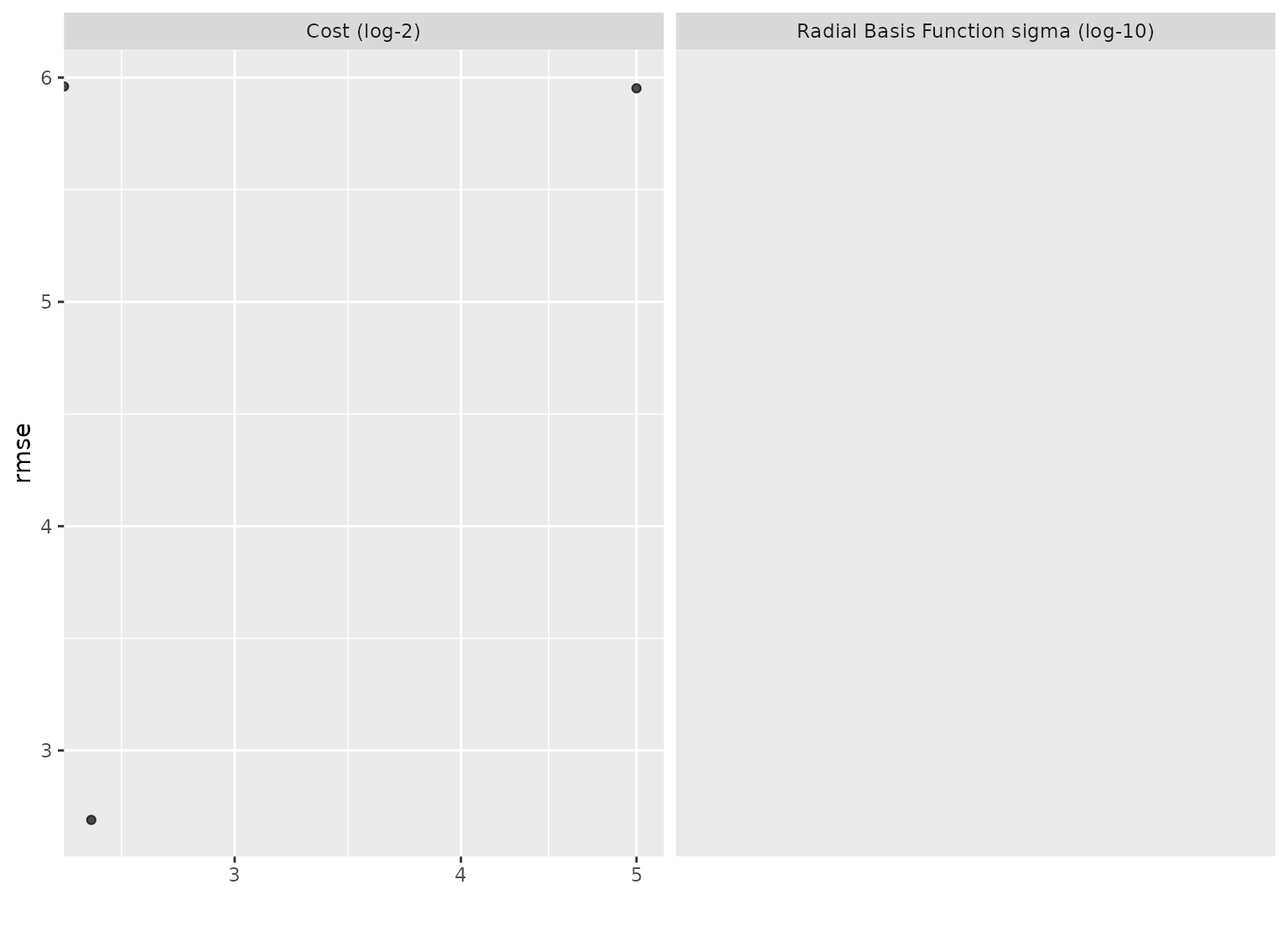
autoplot(svm_res, metric = "rmse") +
  scale_x_log10()
#> Warning: NaNs produced
#> Warning: log-10 transformation introduced infinite values.
#> Warning: Removed 12 rows containing missing values or values outside the scale
#> range (`geom_point()`).


# ---------------------------------------------------------------------------

# Using a variables preprocessor with a workflow

# Rather than supplying a preprocessor (like a recipe) and a model directly
# to `tune_grid()`, you can also wrap them up in a workflow and pass
# that along instead (note that this doesn't do any preprocessing to
# the variables, it passes them along as-is).
wf <- workflow() %>%
  add_variables(outcomes = mpg, predictors = everything()) %>%
  add_model(svm_mod)

set.seed(3254)
svm_res_wf <- tune_grid(wf, resamples = folds, grid = 7)