Introduction
The tune package helps optimize the modeling process. Users can tag arguments in recipes and model objects for optimization. The search routines in tune can discover these arguments and evaluate candidate values until a combination with good performance is found.
As an example, let’s model the Ames housing data:
library(tidymodels)

data(ames)

set.seed(4595)
data_split <- ames %>%
  mutate(Sale_Price = log10(Sale_Price)) %>%
  initial_split(strata = Sale_Price)
ames_train <- training(data_split)
ames_test  <- testing(data_split)
For simplicity, the sale price of a house will be modeled as a function of its geo-location. These predictors appear to have nonlinear relationships with the outcome:
ames_train %>%
  dplyr::select(Sale_Price, Longitude, Latitude) %>%
  tidyr::pivot_longer(cols = c(Longitude, Latitude),
                      names_to = "predictor", values_to = "value") %>%
  ggplot(aes(x = value, Sale_Price)) +
  geom_point(alpha = .2) +
  geom_smooth(se = FALSE) +
  facet_wrap(~ predictor, scales = "free_x")
#> `geom_smooth()` using method = 'gam' and formula 'y ~ s(x, bs = "cs")'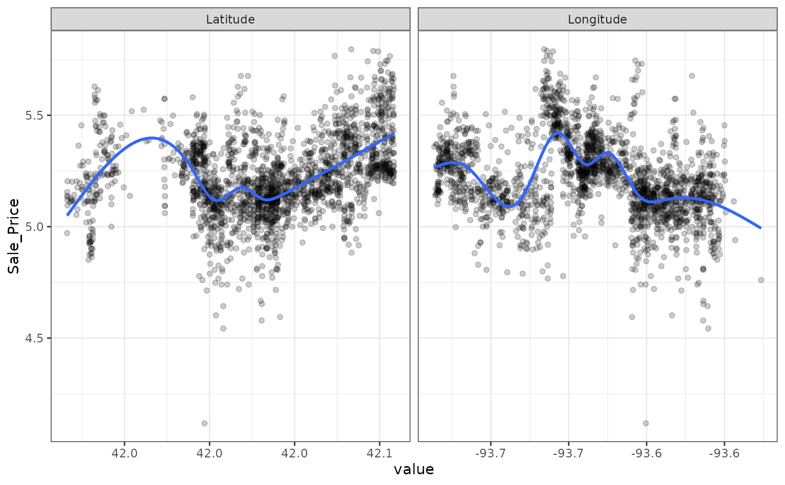
These two predictors could be modeled using natural splines in conjunction with a linear model. The amount of “wiggliness” in these splines is determined by the degrees of freedom. An appropriate value of this parameter cannot be analytically determined from the data, so it is a tuning parameter (a.k.a. a hyper-parameter). A common approach is to use resampling to estimate model performance over different values of these parameters and use these results to set reasonable values.
We can tag these parameters for optimization using the tune() function:
ames_rec <-
  recipe(Sale_Price ~ Gr_Liv_Area + Longitude + Latitude, data = ames_train) %>%
  step_log(Gr_Liv_Area, base = 10) %>%
  step_ns(Longitude, Latitude, deg_free = tune())
The package can detect these values and optimize them.
However, based on the plot above, the potential amount of non-linearity between the sale price and the predictors might be different. For example, longitude might require more flexibility than latitude. The recipe above would constrain the nonlinearity of the predictors to be the same. We can probably do better than that.
To accomplish this, individual step_ns() terms can be added to the recipe for each predictor. However, we want these to be identifiable; using the same syntax as above, we can’t tell the difference between the two deg_free parameters.
tune() has an option to provide a text annotation so that each tuning parameter has a unique identifier:
ames_rec <-
  recipe(Sale_Price ~ Gr_Liv_Area + Longitude + Latitude, data = ames_train) %>%
  step_log(Gr_Liv_Area, base = 10) %>%
  step_ns(Longitude, deg_free = tune("long df")) %>%
  step_ns(Latitude,  deg_free = tune("lat df"))
The function dials::parameters() that can detect and collect the parameters that have been flagged for tuning:
parameters(ames_rec)
#> Collection of 2 parameters for tuning
#>
#>  identifier     type    object
#>     long df deg_free nparam[+]
#>      lat df deg_free nparam[+]
The dials package has default ranges for many parameters. The generic parameter function for deg_free has a fairly small range:
deg_free()
#> Degrees of Freedom (quantitative)
#> Range: [1, 5]
but there is a dials function that is more appropriate for splines:
spline_degree()
#> Piecewise Polynomial Degree (quantitative)
#> Range: [1, 10]
The parameter objects can be easily changed using the update() function:
ames_param <-
  ames_rec %>%
  parameters() %>%
  update(
    `long df` = spline_degree(),
    `lat df` = spline_degree()
  )
ames_param
#> Collection of 2 parameters for tuning
#>
#>  identifier     type    object
#>     long df deg_free nparam[+]
#>      lat df deg_free nparam[+]
Grid Search
Grid search uses a pre-defined set of candidate parameters and evaluates these using resampling. The basic ingredients are:
A grid of candidate values to evaluate.
One or more performance metrics for quantifying how well the model works.
A resampling scheme that can be used to appropriately measure performance (which could be a simple validation set).
To make the grid, a data frame is needed with column names matching the “id” column above. There are several dials functions to created grids (named grid_*). For example, a space-filling design can be created by:
spline_grid <- grid_max_entropy(ames_param, size = 10)
spline_grid
#> # A tibble: 10 x 2
#>    `long df` `lat df`
#>        <int>    <int>
#>  1         6        5
#>  2         7        1
#>  3        10        2
#>  4         3        1
#>  5         1        9
#>  6         9        6
#>  7         1        4
#>  8         3        7
#>  9         9       10
#> 10         5        9
Alternately, expand.grid() also works to create a regular grid:
df_vals <- seq(2, 18, by = 2)
# A regular grid:
spline_grid <- expand.grid(`long df` = df_vals, `lat df` = df_vals)
Note that a 2-degree-of-freedom model is a simple quadratic fit.
There are two other ingredients that are required before tuning.
First is a model specification. Using parsnip, a basic linear model can be used:
lm_mod <- linear_reg() %>% set_engine("lm")No tuning parameters here.
As mentioned above, a resampling specification is also needed. The Ames data set are large enough to use simple 10-fold cross-validation:
The root mean squared error will be used to measure performance (and this is the default for regression problems).
Using these objects, tune_grid() can be used1:
ames_res <- tune_grid(lm_mod, ames_rec, resamples = cv_splits, grid = spline_grid)The object is similar to the rsample object but with one or more extra columns:
ames_res
#> # Tuning results
#> # 10-fold cross-validation using stratification
#> # A tibble: 10 x 4
#>    splits             id     .metrics           .notes
#>    <list>             <chr>  <list>             <list>
#>  1 <split [1976/221]> Fold01 <tibble [162 × 6]> <tibble [0 × 1]>
#>  2 <split [1976/221]> Fold02 <tibble [162 × 6]> <tibble [0 × 1]>
#>  3 <split [1976/221]> Fold03 <tibble [162 × 6]> <tibble [0 × 1]>
#>  4 <split [1976/221]> Fold04 <tibble [162 × 6]> <tibble [0 × 1]>
#>  5 <split [1977/220]> Fold05 <tibble [162 × 6]> <tibble [0 × 1]>
#>  6 <split [1977/220]> Fold06 <tibble [162 × 6]> <tibble [0 × 1]>
#>  7 <split [1978/219]> Fold07 <tibble [162 × 6]> <tibble [0 × 1]>
#>  8 <split [1978/219]> Fold08 <tibble [162 × 6]> <tibble [0 × 1]>
#>  9 <split [1979/218]> Fold09 <tibble [162 × 6]> <tibble [0 × 1]>
#> 10 <split [1980/217]> Fold10 <tibble [162 × 6]> <tibble [0 × 1]>
The .metrics column has all of the holdout performance estimates2 for each parameter combination:
ames_res$.metrics[[1]]
#> # A tibble: 162 x 6
#>    `long df` `lat df` .metric .estimator .estimate .config
#>        <dbl>    <dbl> <chr>   <chr>          <dbl> <chr>
#>  1         2        2 rmse    standard      0.0985 Preprocessor01_Model1
#>  2         2        2 rsq     standard      0.683  Preprocessor01_Model1
#>  3         4        2 rmse    standard      0.0985 Preprocessor02_Model1
#>  4         4        2 rsq     standard      0.683  Preprocessor02_Model1
#>  5         6        2 rmse    standard      0.0973 Preprocessor03_Model1
#>  6         6        2 rsq     standard      0.690  Preprocessor03_Model1
#>  7         8        2 rmse    standard      0.0962 Preprocessor04_Model1
#>  8         8        2 rsq     standard      0.697  Preprocessor04_Model1
#>  9        10        2 rmse    standard      0.0960 Preprocessor05_Model1
#> 10        10        2 rsq     standard      0.699  Preprocessor05_Model1
#> # … with 152 more rows
To get the average metric value for each parameter combination, collect_metrics() can be put to use:
estimates <- collect_metrics(ames_res)
estimates
#> # A tibble: 162 x 8
#>    `long df` `lat df` .metric .estimator   mean     n std_err .config
#>        <dbl>    <dbl> <chr>   <chr>       <dbl> <int>   <dbl> <chr>
#>  1         2        2 rmse    standard   0.100     10 0.00145 Preprocessor01_Mo…
#>  2         2        2 rsq     standard   0.674     10 0.00777 Preprocessor01_Mo…
#>  3         4        2 rmse    standard   0.100     10 0.00153 Preprocessor02_Mo…
#>  4         4        2 rsq     standard   0.675     10 0.00814 Preprocessor02_Mo…
#>  5         6        2 rmse    standard   0.0994    10 0.00161 Preprocessor03_Mo…
#>  6         6        2 rsq     standard   0.680     10 0.00885 Preprocessor03_Mo…
#>  7         8        2 rmse    standard   0.0989    10 0.00159 Preprocessor04_Mo…
#>  8         8        2 rsq     standard   0.684     10 0.00946 Preprocessor04_Mo…
#>  9        10        2 rmse    standard   0.0990    10 0.00165 Preprocessor05_Mo…
#> 10        10        2 rsq     standard   0.683     10 0.0101  Preprocessor05_Mo…
#> # … with 152 more rows
The values in the mean column are the averages of the 10 resamples. The best RMSE values corresponded to:
rmse_vals <-
  estimates %>%
  dplyr::filter(.metric == "rmse") %>%
  arrange(mean)
rmse_vals
#> # A tibble: 81 x 8
#>    `long df` `lat df` .metric .estimator   mean     n std_err .config
#>        <dbl>    <dbl> <chr>   <chr>       <dbl> <int>   <dbl> <chr>
#>  1        16       12 rmse    standard   0.0948    10 0.00120 Preprocessor53_Mo…
#>  2        18       12 rmse    standard   0.0948    10 0.00121 Preprocessor54_Mo…
#>  3        16        8 rmse    standard   0.0949    10 0.00118 Preprocessor35_Mo…
#>  4        16       10 rmse    standard   0.0949    10 0.00118 Preprocessor44_Mo…
#>  5        16       18 rmse    standard   0.0949    10 0.00119 Preprocessor80_Mo…
#>  6        16       16 rmse    standard   0.0949    10 0.00122 Preprocessor71_Mo…
#>  7        18       10 rmse    standard   0.0949    10 0.00119 Preprocessor45_Mo…
#>  8        18        8 rmse    standard   0.0949    10 0.00119 Preprocessor36_Mo…
#>  9        18       18 rmse    standard   0.0950    10 0.00120 Preprocessor81_Mo…
#> 10        16       14 rmse    standard   0.0950    10 0.00117 Preprocessor62_Mo…
#> # … with 71 more rows
Smaller degrees of freedom values correspond to more linear functions, but the grid search indicates that more nonlinearity is better. What was the relationship between these two parameters and RMSE?
autoplot(ames_res, metric = "rmse")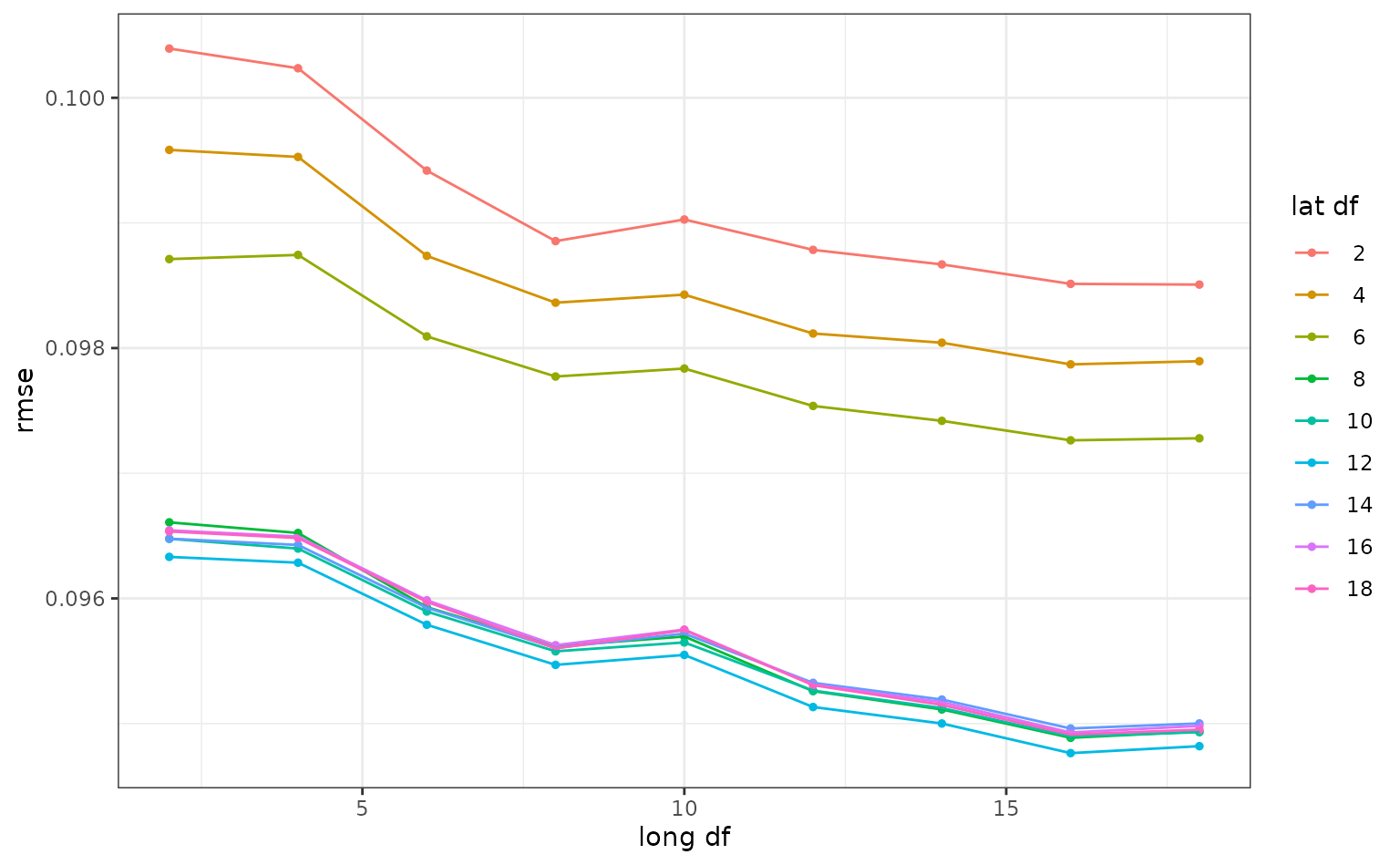
Interestingly, latitude does not do well with degrees of freedom less than 8. How nonlinear are the optimal degrees of freedom?
Let’s plot these spline functions over the data for booth good and bad values of deg_free:
ames_train %>%
  dplyr::select(Sale_Price, Longitude, Latitude) %>%
  tidyr::pivot_longer(cols = c(Longitude, Latitude),
                      names_to = "predictor", values_to = "value") %>%
  ggplot(aes(x = value, Sale_Price)) +
  geom_point(alpha = .2) +
  geom_smooth(se = FALSE, method = lm, formula = y ~ splines::ns(x, df = 3),  col = "red")  +
  geom_smooth(se = FALSE, method = lm, formula = y ~ splines::ns(x, df = 16)) +
  scale_y_log10() +
  facet_wrap(~ predictor, scales = "free_x")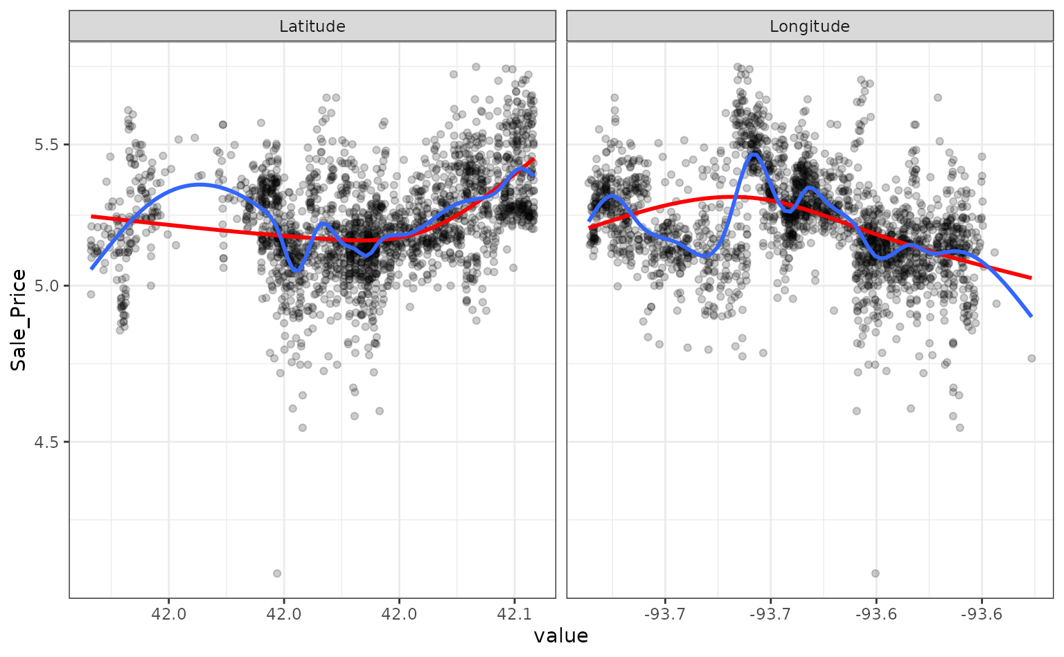
Looking at these plots, the smaller degrees of freedom (red) are clearly under-fitting. Visually, the more complex splines (blue) might indicate that there is overfitting but this would result in poor RMSE values when computed on the hold-out data.
Based on these results, a new recipe would be created with the optimized values (using the entire training set) and this would be combined with a linear model created form the entire training set.
Model Optimization
Instead of a linear regression, a nonlinear model might provide good performance. A K-nearest-neighbor fit will also be optimized. For this example, the number of neighbors and the distance weighting function will be optimized:
# requires the kknn package
knn_mod <-
  nearest_neighbor(neighbors = tune(), weight_func = tune()) %>%
  set_engine("kknn") %>%
  set_mode("regression")
The easiest approach to optimize the pre-processing and model parameters is to bundle these objects into a workflow:
library(workflows)
knn_wflow <-
  workflow() %>%
  add_model(knn_mod) %>%
  add_recipe(ames_rec)
From this, the parameter set can be used to modify the range and values of parameters being optimized3:
knn_param <-
  knn_wflow %>%
  parameters() %>%
    update(
    `long df` = spline_degree(c(2, 18)),
    `lat df` = spline_degree(c(2, 18)),
    neighbors = neighbors(c(3, 50)),
    weight_func = weight_func(values = c("rectangular", "inv", "gaussian", "triangular"))
  )
This parameter collection can be passed to the grid functions via the param_info arguments.
Instead of using grid search, an iterative method called Bayesian optimization can be used. This takes an initial set of results and tries to predict the next tuning parameters to evaluate.
Although no grid is required, the process requires a few additional pieces of information:
A description of the search space. At a minimum, the would consist of ranges for numeric values and a list of values for categorical tuning parameters.
An acquisition function that helps score potential tuning parameter values.
A model for analyzing and making predictions of the best tuning parameter values. A Gaussian Process model is typical and used here.
The code to conduct the search is:
ctrl <- control_bayes(verbose = TRUE)
set.seed(8154)
knn_search <- tune_bayes(knn_wflow, resamples = cv_splits, initial = 5, iter = 20,
                         param_info = knn_param, control = ctrl)
#>
#> ❯  Generating a set of 5 initial parameter results
#> ✓ Initialization complete
#>
#> Optimizing rmse using the expected improvement
#>
#> ── Iteration 1 ─────────────────────────────────────────────────────────────────
#>
#> i Current best:      rmse=0.08576 (@iter 0)
#> i Gaussian process model
#> ! The Gaussian process model is being fit using 7 features but only has 5
#>   data points to do so. This may cause errors or a poor model fit.
#> ✓ Gaussian process model
#> i Generating 4773 candidates
#> i Predicted candidates
#> i neighbors=3, weight_func=triangular, long df=2, lat df=18
#> i Estimating performance
#> ✓ Estimating performance
#> ⓧ Newest results:    rmse=0.09449 (+/-0.00136)
#>
#> ── Iteration 2 ─────────────────────────────────────────────────────────────────
#>
#> i Current best:      rmse=0.08576 (@iter 0)
#> i Gaussian process model
#> ! The Gaussian process model is being fit using 7 features but only has 6
#>   data points to do so. This may cause errors or a poor model fit.
#> ✓ Gaussian process model
#> i Generating 4769 candidates
#> i Predicted candidates
#> i neighbors=10, weight_func=triangular, long df=7, lat df=10
#> i Estimating performance
#> ✓ Estimating performance
#> ♥ Newest results:    rmse=0.08265 (+/-0.00208)
#>
#> ── Iteration 3 ─────────────────────────────────────────────────────────────────
#>
#> i Current best:      rmse=0.08265 (@iter 2)
#> i Gaussian process model
#> ! The Gaussian process model is being fit using 7 features but only has 7
#>   data points to do so. This may cause errors or a poor model fit.
#> ✓ Gaussian process model
#> i Generating 4776 candidates
#> i Predicted candidates
#> i neighbors=6, weight_func=triangular, long df=6, lat df=18
#> i Estimating performance
#> ✓ Estimating performance
#> ⓧ Newest results:    rmse=0.08724 (+/-0.00175)
#>
#> ── Iteration 4 ─────────────────────────────────────────────────────────────────
#>
#> i Current best:      rmse=0.08265 (@iter 2)
#> i Gaussian process model
#> ! The Gaussian process model is being fit using 7 features but only has 8
#>   data points to do so. This may cause errors or a poor model fit.
#> ✓ Gaussian process model
#> i Generating 4765 candidates
#> i Predicted candidates
#> i neighbors=44, weight_func=gaussian, long df=7, lat df=2
#> i Estimating performance
#> ✓ Estimating performance
#> ⓧ Newest results:    rmse=0.08992 (+/-0.0016)
#>
#> ── Iteration 5 ─────────────────────────────────────────────────────────────────
#>
#> i Current best:      rmse=0.08265 (@iter 2)
#> i Gaussian process model
#> ✓ Gaussian process model
#> i Generating 4787 candidates
#> i Predicted candidates
#> i neighbors=9, weight_func=triangular, long df=7, lat df=2
#> i Estimating performance
#> ✓ Estimating performance
#> ⓧ Newest results:    rmse=0.08438 (+/-0.00148)
#>
#> ── Iteration 6 ─────────────────────────────────────────────────────────────────
#>
#> i Current best:      rmse=0.08265 (@iter 2)
#> i Gaussian process model
#> ✓ Gaussian process model
#> i Generating 4792 candidates
#> i Predicted candidates
#> i neighbors=4, weight_func=inv, long df=7, lat df=10
#> i Estimating performance
#> ✓ Estimating performance
#> ⓧ Newest results:    rmse=0.08509 (+/-0.00215)
#>
#> ── Iteration 7 ─────────────────────────────────────────────────────────────────
#>
#> i Current best:      rmse=0.08265 (@iter 2)
#> i Gaussian process model
#> ✓ Gaussian process model
#> i Generating 4775 candidates
#> i Predicted candidates
#> i neighbors=32, weight_func=triangular, long df=7, lat df=8
#> i Estimating performance
#> ✓ Estimating performance
#> ⓧ Newest results:    rmse=0.08643 (+/-0.00195)
#>
#> ── Iteration 8 ─────────────────────────────────────────────────────────────────
#>
#> i Current best:      rmse=0.08265 (@iter 2)
#> i Gaussian process model
#> ✓ Gaussian process model
#> i Generating 4769 candidates
#> i Predicted candidates
#> i neighbors=3, weight_func=rectangular, long df=7, lat df=13
#> i Estimating performance
#> ✓ Estimating performance
#> ⓧ Newest results:    rmse=0.08874 (+/-0.00189)
#>
#> ── Iteration 9 ─────────────────────────────────────────────────────────────────
#>
#> i Current best:      rmse=0.08265 (@iter 2)
#> i Gaussian process model
#> ✓ Gaussian process model
#> i Generating 4771 candidates
#> i Predicted candidates
#> i neighbors=17, weight_func=inv, long df=7, lat df=9
#> i Estimating performance
#> ✓ Estimating performance
#> ⓧ Newest results:    rmse=0.08438 (+/-0.0019)
#>
#> ── Iteration 10 ────────────────────────────────────────────────────────────────
#>
#> i Current best:      rmse=0.08265 (@iter 2)
#> i Gaussian process model
#> ✓ Gaussian process model
#> i Generating 4742 candidates
#> i Predicted candidates
#> i neighbors=14, weight_func=triangular, long df=7, lat df=9
#> i Estimating performance
#> ✓ Estimating performance
#> ⓧ Newest results:    rmse=0.08311 (+/-0.00202)
#>
#> ── Iteration 11 ────────────────────────────────────────────────────────────────
#>
#> i Current best:      rmse=0.08265 (@iter 2)
#> i Gaussian process model
#> ✓ Gaussian process model
#> i Generating 4752 candidates
#> i Predicted candidates
#> i neighbors=9, weight_func=gaussian, long df=7, lat df=16
#> i Estimating performance
#> ✓ Estimating performance
#> ⓧ Newest results:    rmse=0.08704 (+/-0.00225)
#>
#> ── Iteration 12 ────────────────────────────────────────────────────────────────
#>
#> i Current best:      rmse=0.08265 (@iter 2)
#> i Gaussian process model
#> ✓ Gaussian process model
#> i Generating 4779 candidates
#> i Predicted candidates
#> i neighbors=9, weight_func=triangular, long df=7, lat df=13
#> i Estimating performance
#> ✓ Estimating performance
#> ⓧ Newest results:    rmse=0.08397 (+/-0.002)
#> ! No improvement for 10 iterations; returning current results.
Visually, the performance gain was:
autoplot(knn_search, type = "performance", metric = "rmse")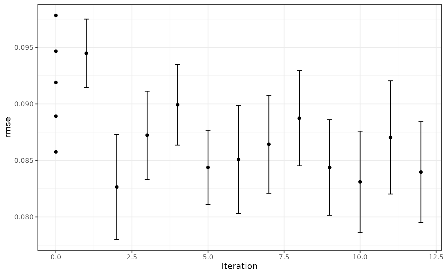
The best results here were:
collect_metrics(knn_search) %>%
  dplyr::filter(.metric == "rmse") %>%
  arrange(mean)
#> # A tibble: 17 x 11
#>    neighbors weight_func `long df` `lat df` .metric .estimator   mean     n
#>        <int> <chr>           <int>    <int> <chr>   <chr>       <dbl> <int>
#>  1        10 triangular          7       10 rmse    standard   0.0827    10
#>  2        14 triangular          7        9 rmse    standard   0.0831    10
#>  3         9 triangular          7       13 rmse    standard   0.0840    10
#>  4        17 inv                 7        9 rmse    standard   0.0844    10
#>  5         9 triangular          7        2 rmse    standard   0.0844    10
#>  6         4 inv                 7       10 rmse    standard   0.0851    10
#>  7         5 triangular          8       14 rmse    standard   0.0858    10
#>  8        32 triangular          7        8 rmse    standard   0.0864    10
#>  9         9 gaussian            7       16 rmse    standard   0.0870    10
#> 10         6 triangular          6       18 rmse    standard   0.0872    10
#> 11         3 rectangular         7       13 rmse    standard   0.0887    10
#> 12        36 triangular          9        6 rmse    standard   0.0889    10
#> 13        44 gaussian            7        2 rmse    standard   0.0899    10
#> 14        28 inv                16       10 rmse    standard   0.0919    10
#> 15         3 triangular          2       18 rmse    standard   0.0945    10
#> 16        18 rectangular        13        3 rmse    standard   0.0947    10
#> 17        47 inv                 3       16 rmse    standard   0.0978    10
#> # … with 3 more variables: std_err <dbl>, .config <chr>, .iter <int>
With this intrinsically nonlinear model there is less reliance on the nonlinear terms created by the recipe.
A simple R model formula could have been used here, such as
Sale_Price ~ log10(Gr_Liv_Area) + Longitude + Latitude. A recipe is not required.↩︎tunehas default measures of performance that it uses if none are specified. Here the RMSE and R2 are estimated. This can be changed using themetricsoption.↩︎One of the tuning parameters (
weight_func) is categorical and, by default, has 10 unique values. The model used to predict new test parameters is a Gaussian process model, and this can become slow to fit when the number of tuning parameters is large or when a categorical parameter generates many dummy variables. We’ve reduced the number of categories for this parameter to speed things up a bit.↩︎